From Prior Beliefs to Posterior Inference
We saw in the previous section that to inference based on maximum likelihood estimation returns disappointing results, even in the instance where we introduce hard constraints on the possible realistic parameter values.
In this section we look at how this hard assumption about the plausible total number of socks can be replaced with a softer appraoch where we specify our belief about the total number as a distribution. This distribution is specified independently of the observed data (eg. in this case we do not factor in the observation of \(k = 11\) distinct socks), and as such it is called the prior distribution as it represents our beliefs prior to seeing any data.
We will then explain how we can derive a distribution for the number of socks which takes into account both our prior belief, and the observed data; this will be the posterior distribution, and is fully determined by combining the prior with the likelihood function.
This method of having a structured way of accounting for prior knowledge in statistics is often considered the central benefit (or detriment, depending on your school of thought) of Bayesian analysis. It is worth noting, however, that there are subtler distinctions that
Bayes theorem will enable us to combine
One of the distinctions between the Bayesian approach to statistics and alternative schools of thought (eg. frequentist) is the The Bayesian approach to statistics differs from the
socks_bayes <- function(p_max = 50, s_max = 50, k = 11, log_likelihood = NULL, log_prior = NULL){

  if(is.null(log_prior)){

    warning("Warning: Defaulting to the constant prior; this may yield an improper posterior.")

    log_prior <- function(p,s){1}
    log_prior <- Vectorize(log_prior)
    }

  socks <- crossing(data_frame(p = 0:p_max), data_frame(s = 0:s_max)) %>%
    mutate(
      n = 2*p + s,
      k = k,

      log_likelihood = log_likelihood(p,s,k),
      log_prior = log_prior(p,s),
      prior = exp(log_prior),

      log_posterior_tilde = log_prior + log_likelihood,

      log_posterior_tilde = log_posterior_tilde - max(log_posterior_tilde),

      posterior_tilde = exp(log_posterior_tilde),
      posterior = posterior_tilde / sum(posterior_tilde),

      log_posterior = log(posterior)
  )

  socks <- socks %>% select(p,s,n,k, log_prior, log_likelihood, prior, log_posterior, posterior)

  return(socks)
}
Bååth’s Prior
Our first analysis will replicate that conducted by Bååth, who constructs the prior on \((p,s)\) as follows.
Defining the Prior
First a prior is placed on \(n\), the overall total number of socks that are believed to be in the washing machine. He chooses to use a negative binomial distribution. Bååth chooses parameters for this distribution based on prior knowledge that Broman is one in a family of four, and a belief that Broman only runs one wash per week, and as such decided to use a negative binomial distribution with mean \(\mu = 30\) (corresponding to 15 pairs of socks), with a standard deviation of \(\sigma = 15\); we denote this distribution by \(P_{\mu,\sigma}(n)\).
prior_n <- function(n, mu = 30, sigma = 15){

  size <- -mu^2 / (mu - sigma^2)

  prior_prob <- dnbinom(n, mu = mu, size = size)

  return(prior_prob)
}
## Warning: `data_frame()` is deprecated as of tibble 1.1.0.
## Please use `tibble()` instead.
## This warning is displayed once every 8 hours.
## Call `lifecycle::last_warnings()` to see where this warning was generated.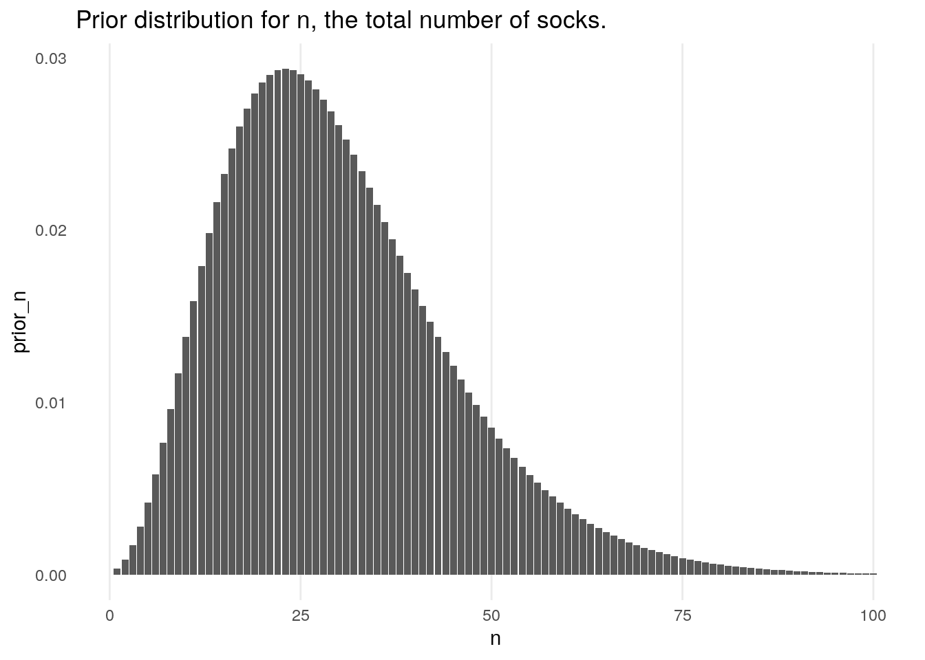
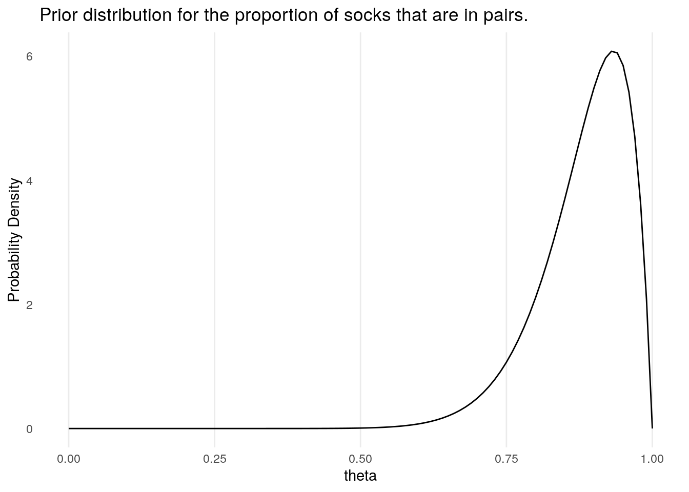
Having determined the total number of socks that he expects there to be in any given wash, Bååth then uses a prior for the proportion of socks that are pairs, as opposed to singletons. Denoting this proportion \(\theta = 2p/(2p + s)\), Bååth places on this a Beta prior (the natural choice for a proportion measure between 0 and 1). This has prior parameters \(\alpha\), \(\beta\) which are chosen to be \(\alpha = 15, \, \beta = 2\), which were chosen to conform with his own laundry habits. We will denote this distribution by \(P_{\alpha,\beta}(\theta)\).
We now have to work out how to turn priors on \(n\) and \(\theta\) into priors for \(p,s\); this is handled fairly easily in Bååth’s original computation approach through a sampling process:
- Sample \(n\), and \(\theta\) from the respective prior distributions defined above.
- Let \(p = \left[ \theta \rfloor n/2 \lfloor \right]\), where \(\rfloor x \lfloor\) denotes the floor of \(x\), and \(\left[x\right]\) denotes \(x\) rounded to the nearest integer.
- Let \(s = n - 2p\).
Without providing full details, following these steps mathematically leads to the following formula for the prior distribution of \((p,s)\)
\[ P(p,s) = P_{\mu,\sigma}(2p+s) \left\{ F_{\alpha,\beta}\left(\frac{2p +1}{2\lfloor p + s/2 \rfloor}\right) - F_{\alpha,\beta}\left(\frac{2p -1}{2\lfloor p + s/2 \rfloor}\right) \right\}, \] where \(F_{\alpha,\beta}(t) = P_{\alpha, \beta}(\theta \leq t)\) is the cummulative density of the Beta distribution; the term in braces corresponds to the probability that \(\theta\) lies in the range of values that when multiplied by \(2p + s\), and rounded to the nearest integer returns the answer of \(p\).
We define the prior below
log_prior_baath <- function(p,s, mu = 30, sigma = 15, alpha = 15, beta = 2){

  if(min(alpha,beta) == 0 & s > 0){
    return(-Inf)
  }

  n <- 2*p + s

  prior_n <- prior_n(n, mu, sigma)

  theta_hgh <- (2*p + 1)/(2 * floor(n/2) )
  theta_low <- (2*p - 1)/(2 * floor(n/2) )

  theta_hgh <- (theta_hgh %>% max(.,0)) %>% min(.,1)
  theta_low <- (theta_low %>% max(.,0)) %>% min(.,1)

  prior_theta <-pbeta(theta_hgh, shape1 = alpha, shape2 = beta) - pbeta(theta_low, shape1 = alpha, shape2 = beta)

  return( log(prior_n) + log(prior_theta))
}

log_prior_baath <- Vectorize(log_prior_baath)
The 2D density plot below shows how the prior distribution varies over combinations of (2p,s); the highest density goes to the scenario in which there are a total of 19 socks, made up of \(p = 8\) pairs and \(s = 3\) singletons. 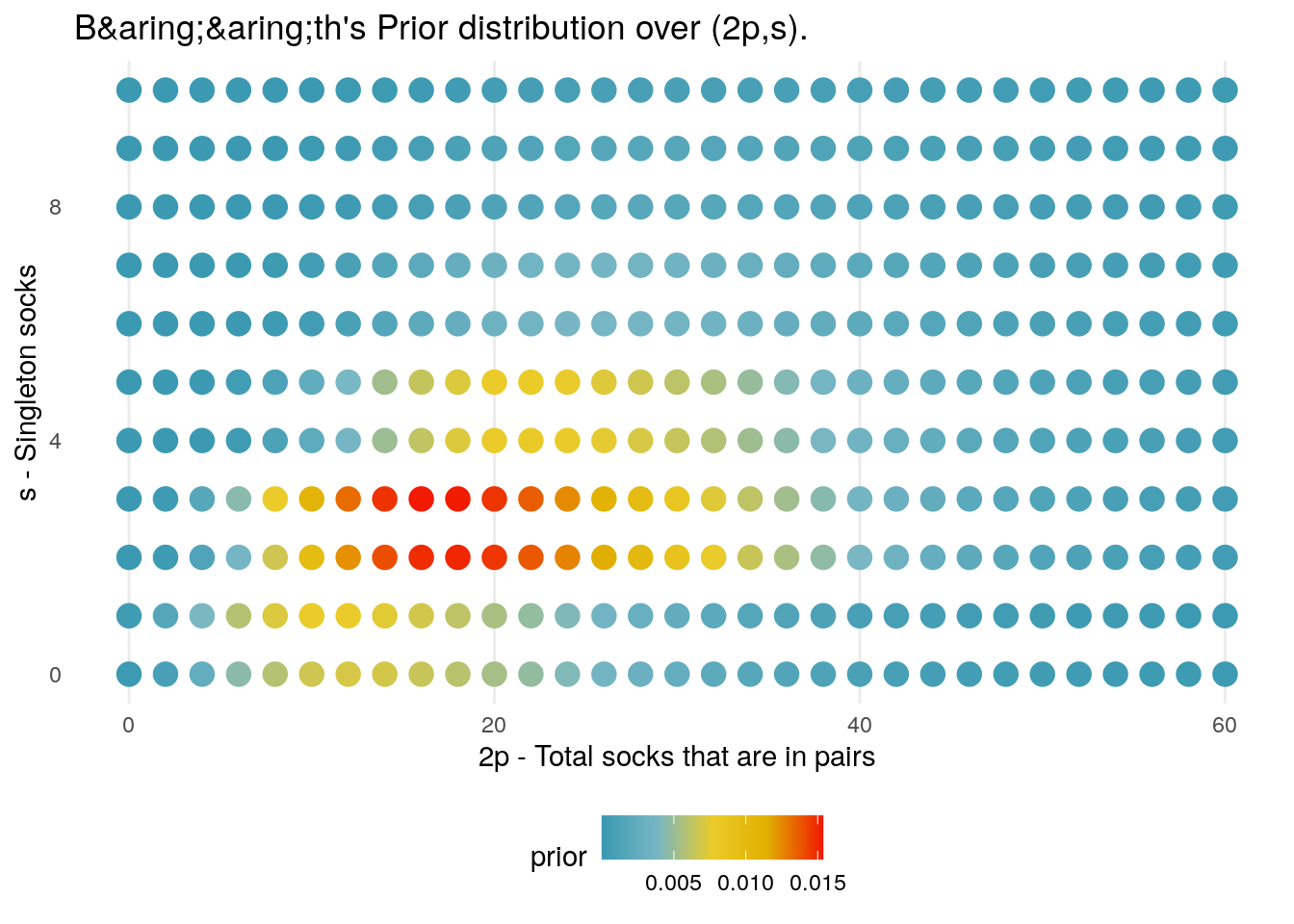
knitr::knit_exit()